Tutorial 1 - Harvest projection • salmonMSE

Operating model basics

This tutorial is an introduction to the basic mechanics of working with the salmonMSE projection model.

The operating model is an object where we put parameters describing the life history of our case study and the management strategy to be evaluated.

In R, the operating model is an S4 object of class SOM. We can view the documentation with:

library(salmonMSE)
class?SOM

The SOM object is built out of constituent objects that organizes the inputs and different management levers. Creating a full SOM looks something like this:

# Note: demonstration only, this code chunk will not work
SOM <- new(
  "SOM",
  Bio = Bio,
  Habitat = Habitat,
  Hatchery = Hatchery,
  Harvest = Harvest,
  Historical = Historical
)

We’ll work with 5 smaller objects (Bio, Habitat, Hatchery, Harvest, and Historical), each of which are S4 objects with pre-defined input slots. Each also has its own documentation page with the necessary description and dimensions of the input object (arrays, matrices, etc). For example, access the documentation for the Bio object with:

class?Bio

While we need to create all five objects, we may carefully work with as few as 1-2 objects depending on the case study, but others may not be relevant, for example, we are not evaluating hatchery production.

Let’s start simple with a model that implements a fishery harvest rate.

Simple case study

Bio object

The Bio object component of the operating model describes the basic biology (maturity, lifespan) of the population. In general, we need to describe what happens in each age class.

Here’s the first example, where we will fill in the slots in line-by-line:

nsim <- 20
SAR <- 0.01

set.seed(4389)
kappa_mean <- 3
kappa_sd <- 0.5

kappa <- EnvStats::rnormTrunc(nsim, kappa_mean, kappa_sd, min = 1, max = Inf)

Bio <- new("Bio")
Bio@Name <- "Prototype"
Bio@maxage <- 3
Bio@p_mature <- c(0, 0, 1)
Bio@SRrel <- "Ricker"
Bio@kappa <- kappa
Bio@Smax <- 1000
Bio@Mjuv_NOS <- c(0, -log(SAR))
Bio@fec <- c(0, 0, 5000)
Bio@p_female <- 0.5

Alternatively, the Bio object can be filled in one call:

nsim <- 20
SAR <- 0.01

set.seed(4389)
kappa_mean <- 3
kappa_sd <- 0.5

kappa <- EnvStats::rnormTrunc(nsim, kappa_mean, kappa_sd, min = 1, max = Inf)

Bio <- new(
  Class = "Bio",
  maxage = 3,
  p_mature = c(0, 0, 1),
  SRrel = "Ricker",
  kappa = kappa,
  Smax = 1000,
  Mjuv_NOS = c(0, -log(SAR)),
  fec = c(0, 0, 5000),
  p_female = 0.5
)

The information contained in this object:

The lifespan is 3 years
All fish mature at age 3
Natural-origin juvenile marine survival is 0.01, occurring between age 2 to 3
50% of spawners are female, each with fecundity of 5 thousand eggs
The density-dependence of the population is described with a Ricker stock-recruit function. The productivity parameter (kappa) is stochastic over 20 simulations with an average of 3 adults/spawner. The Smax parameter is 1,000 spawners.

There’s also some other default parameters that we are not discussing (for example, en-route survival to spawning grounds is 1, see class?Bio).

Harvest object

In the Bio object, we have egg-juvenile survival described in the Ricker stock recruit relationship, and juvenile marine survival is 0.01.

Next, we describe the exploitation rate in the fishery in the Harvest object:

Harvest <- new(
  "Harvest",
  u_preterminal = 0,
  u_terminal = 0.2,
  vulT = c(1, 1, 1)
)

The information in this object:

There is no preterminal marine fishery exploitation, i.e., fishing on juveniles
The terminal exploitation rate is 0.2
The terminal fishery selects all ages equally (vulnerability is identical for all ages, but note that only age-3 fish return and are available to the fishery in the first place).

Other objects

We have to specify the Hatchery, Habitat, and Historical objects. However, we don’t have a hatchery and we don’t model individual freshwater life stages. Thus, our Hatchery, Habitat objects are quite simple:

# Set releases to zero to turn off hatchery
Hatchery <- new(
  "Hatchery",
  n_yearling = 0,
  n_subyearling = 0
)

# Use flag to be explicit about assumptions
Habitat <- new(
  "Habitat",
  use_habitat = FALSE
)

We will simulate with 1,000 juveniles at the start of the projection:

# Set number of juveniles at beginning of simulation
Historical <- new(
  "Historical",
  InitNjuv_NOS = 1000,
  InitNjuv_HOS = 0
)

Run projection

We create the SOM object now that we have individual objects completed:

proyears <- 50 # Specify the number of projection years
SOM <- new(
  "SOM",
  nsim = nsim,
  proyears = proyears,
  Bio = Bio,
  Habitat = Habitat,
  Hatchery = Hatchery,
  Harvest = Harvest,
  Historical = Historical
)

Then, we run the projection with a call to salmonMSE().

Generally, it’s a good idea to save the output, especially for larger models and extensive analyses.

SMSE <- salmonMSE(SOM)
#saveRDS(SMSE, "1-simple.rds")

Reporting

We then generate a markdown report of the projection with report():

report(SMSE)

Exploring output

The output (class SMSE) from the projection contains various arrays of the state variables during the projection. For example, this slot contains the projected natural-origin spawners (NOS) in an array by simulation, stock, age, and year:

SMSE@NOS

All other slots can be found with:

slotNames(SMSE)

The corresponding documentation is found with:

class?SMSE

Figures

There are plotting functions to help us explore the output.

plot_statevar_ts() generates a time series figure with base graphics. By default, it generates line plots for each stochastic simulation in the projection:

plot_statevar_ts(SMSE, "NOS")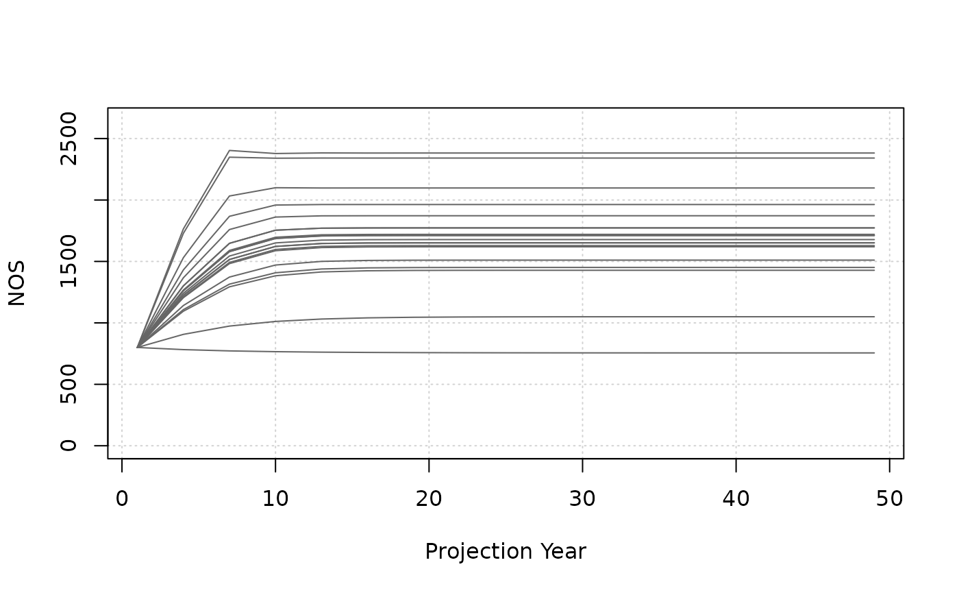

Adding an additional argument gives us a summary quantile by year:

plot_statevar_ts(SMSE, "NOS", quant = TRUE)

We can also explore the distribution of outcomes within an individual year. plot_statevar_hist() returns a histogram. By default, it plots the values in the last year of the projection:

plot_statevar_hist(SMSE, "NOS")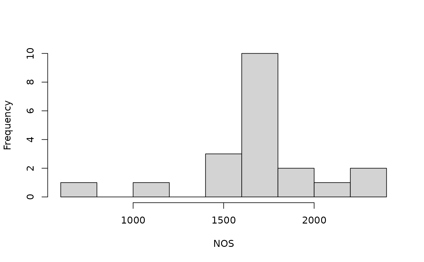

And again, an additional argument gives us control to plot distributions in other projection years:

plot_statevar_hist(SMSE, "NOS", y = 1)

All these figures return results from a single model run. We will explore how to compare model runs in Tutorial 3.

Tutorial 1 - Harvest projection

2026-08-13