Tutorial 3 - Running multiple scenarios (harvest projection)
2026-09-25
Source:vignettes/tutorial-3.Rmd
tutorial-3.RmdMultiple model runs
Here, we demonstrate how to organize an analysis that evaluates alternative management strategies across uncertain biological parameters.
The management strategy to be evaluated is the terminal exploitation rate (ER), which is evaluated in separate simulation runs.
The two uncertain parameters for which we want to evaluate robustness is marine survival (SAR) and the stock-recruit (SR) Ricker parameters. We incorporate uncertainty in Ricker parameters within operating model, while marine survival is specified in separate operating models.
Each operating model is a unique description of the system dynamics. Thus, individual operating models contain separate combinations of ER and marine survival.
The recommended simulation approach is as follows:
- Write the R code that executes a single model run
- Place that code in a wrapper function that will be used to repeat the simulation for various combination of parameters
- Create a grid that identifies all parameter values that will adjusted in the full simulation
- Repeat the simulation over all parameter values. Take advantage of
the parallel processing capabilities and vectorization capabilities of
R, e.g., the
lapply()function.
Once we have completed the simulation, we will have to aggregate the results to compare the outcomes in the grid.
Step 1: Single model run
Below is a single code chunk for a single model projection, using a similar life cycle modeling approach as in Tutorial 1:
library(salmonMSE)
nsim <- 20
set.seed(234)

SAR <- 0.01
ER <- 0.1

# We are sampling Ricker alpha values which represent maximum egg-smolt survival
# While salmonMSE expects productivity values (recruits/spawner) in the kappa slot,
# we can set the phi conversion term to 1 to directly enter alpha
alpha_mean <- 0.1
alpha_sd <- 0.15
alpha <- rlnorm(nsim, log(alpha_mean) - 0.5 * alpha_sd^2, alpha_sd)

# We are sampling Ricker Emax = 1/beta (egg production that maximizes the stock-recruit function)
# represent maximum egg-smolt survival
# While salmonMSE expects Smax,
# we can set both phi and tau conversions term to 1 to directly enter Emax
# Here mean Emax is the egg production from 1000 spawners (fecundity = 5,000 eggs)
Emax_mean <- 1000 * 5000
Emax_sd <- 0.2
Emax <- rlnorm(nsim, log(Emax_mean) - 0.5 * Emax_sd^2, Emax_sd)

Bio <- new(
  Class = "Bio",
  maxage = 3,
  p_mature = c(0, 0, 1),
  SRrel = "Ricker",
  kappa = alpha,
  Smax = Emax,
  phi = 1,
  tau = 1,
  Mjuv_NOS = c(0, -log(SAR)),
  fec = c(0, 0, 5000),
  p_female = 0.5
)

Harvest <- new(
  "Harvest",
  u_preterminal = 0,
  u_terminal = ER,
  vulT = c(1, 1, 1)
)

Hatchery <- new(
  "Hatchery",
  n_yearling = 0,
  n_subyearling = 0
)

# Use flag to be explicit about assumptions
Habitat <- new(
  "Habitat",
  use_habitat = FALSE
)

# Set number of juveniles at beginning of simulation
InitNjuv_NOS <- array(1000, c(nsim, Bio@maxage, 1))
InitNjuv_NOS[, 1:2, ] <- 1000 / SAR
Historical <- new(
  "Historical",
  InitNjuv_NOS = InitNjuv_NOS,
  InitNjuv_HOS = 0
)

proyears <- 40
SOM <- new(
  "SOM",
  nsim = nsim,
  proyears = proyears,
  Bio = Bio,
  Habitat = Habitat,
  Hatchery = Hatchery,
  Harvest = Harvest,
  Historical = Historical
)
SMSE <- salmonMSE(SOM)
Step 2: Wrapper function
Now let’s put the above code chunk into a function. We’ll call it
wrapper().
This function has three arguments:
-
SAR_vectorthat contains a vector of marine survival values -
ER_vectorthat contains a vector of exploitation rate values, same length asSAR_vector -
iwhich is an integer that indexes bothSAR_vectorandER_vector. Whenwrapper()is called, you supply a value foriand the function will grab thei-th value inSAR_vectorandER_vectorfor the model run.
The rest of the function should be the same as the previous chunk. The wrapper function re-creates the same operating model each time the function is called, except for the SAR and ER value, runs the projection, and returns the output to the user:
wrapper <- function(i, SAR_vector, ER_vector) {

  require(salmonMSE)

  SAR <- SAR_vector[i]
  ER <- ER_vector[i]

  nsim <- 20
  set.seed(234)

  # We are sampling Ricker alpha values which represent maximum egg-smolt survival
  # While salmonMSE expects productivity values (recruits/spawner) in the kappa slot,
  # we can set the phi conversion term to 1 to directly enter alpha
  alpha_mean <- 0.1
  alpha_sd <- 0.15
  alpha <- rlnorm(nsim, log(alpha_mean) - 0.5 * alpha_sd^2, alpha_sd)

  # We are sampling Ricker Emax = 1/beta (egg production that maximizes the stock-recruit function)
  # represent maximum egg-smolt survival
  # While salmonMSE expects Smax,
  # we can set both phi and tau conversions term to 1 to directly enter Emax
  # Here mean Emax is the egg production from 1000 spawners (fecundity = 5,000 eggs)
  Emax_mean <- 1000 * 5000
  Emax_sd <- 0.2
  Emax <- rlnorm(nsim, log(Emax_mean) - 0.5 * Emax_sd^2, Emax_sd)

  Bio <- new(
    Class = "Bio",
    maxage = 3,
    p_mature = c(0, 0, 1),
    SRrel = "Ricker",
    kappa = alpha,
    Smax = Emax,
    phi = 1,
    tau = 1,
    Mjuv_NOS = c(0, -log(SAR)),
    fec = c(0, 0, 5000),
    p_female = 0.5
  )

  Harvest <- new(
    "Harvest",
    u_preterminal = 0,
    u_terminal = ER,
    vulT = c(1, 1, 1)
  )

  Hatchery <- new(
    "Hatchery",
    n_yearling = 0,
    n_subyearling = 0
  )

  # Use flag to be explicit about assumptions
  Habitat <- new(
    "Habitat",
    use_habitat = FALSE
  )

  # Set number of juveniles at beginning of simulation
  InitNjuv_NOS <- array(1000, c(nsim, Bio@maxage, 1))
  InitNjuv_NOS[, 1:2, ] <- 1000 / SAR
  Historical <- new(
    "Historical",
    InitNjuv_NOS = InitNjuv_NOS,
    InitNjuv_HOS = 0
  )

  proyears <- 20
  SOM <- new(
    "SOM",
    nsim = nsim,
    proyears = proyears,
    Bio = Bio,
    Habitat = Habitat,
    Hatchery = Hatchery,
    Harvest = Harvest,
    Historical = Historical
  )

  SMSE <- salmonMSE(SOM)

  return(SMSE)
}
Step 3 - Create parameter grid
Before we can use the wrapper function, we create the simulation design, i.e., which ERs and marine survival values we will use.
One way to create a grid of values is with expand.grid()
from separate vectors of marine survival and ERs. Each row identifies a
unique set of values in the grid:
simulation_design <- expand.grid(
  SAR_vector = seq(0.005, 0.03, 0.005),
  ER_vector = seq(0.2, 0.7, 0.1)
)
Step 4: Repeat simulation
Once we have our wrapper function and simulation design, we can now run the simulation.
There’s various ways to run the projections depending on our computation capabilities, e.g., old laptop, new desktop, computing cluster, etc.
Non-parallel computation
We can run a loop over each row of our simulation_design
data frame:
SMSE_list <- list()
for (i in 1:nrow(simulation_design)) {
  SMSE_list[[i]] <- wrapper(
    i,
    SAR_vector = simulation_design$SAR_vector,
    ER_vector = simulation_design$ER_vector
  )
}
The lapply() function has a similar functionality that
repeats calculations down the rows of the simulation grid:
Parallel computation
Loops are computationally slower compared to parallel processing. We
use the parallel package to run simulations over 10 CPUs,
then save the results:
library(parallel)
cpus <- 10

cl <- makeCluster(cpus)

SMSE_list <- parLapply(
  cl,
  X = 1:nrow(simulation_design),
  wrapper,
  SAR_vector = simulation_design$SAR_vector,
  ER_vector = simulation_design$ER_vector
)

stopCluster(cl)
It is also possible to run parallel simulations within a single operating model, for example, with
SMSE <- salmonMSE(SOM, ncores = 10). This feature is probably best suited for individual model runs with many simulation replicates.
Results
Now we have a list of SMSE objects in
SMSE_list.
Compare time series
In Tutorials 1 & 2, we saw that report() generates a
Markdown report from a single model run. Here, we want to compare
several model runs simultaneously in a figure.
We have the compare() function which generates another
markdown report that plots state variables from separate model runs.
We have 36 scenarios, so we may not be able to neatly all into individual figures. Here’s how to compare just the first 3 model runs:
# Create names for each model run by pasting the SAR and ER values
SMSE_names <- paste0("SAR = ", simulation_design$SAR_vector, ", ER = ", simulation_design$ER_vector)

compare(SMSE_list = SMSE_list[1:3], names = SMSE_names[1:3])
compare_statevar_ts() generates a time series figure
with base graphics. While the default settings generate a line plot for
each stochastic simulation, it can quickly get messy.
Let’s directly proceed to quantile figures:
compare_statevar_ts(SMSE_list[1:3], var = "NOS", quant = TRUE, names = SMSE_names[1:3])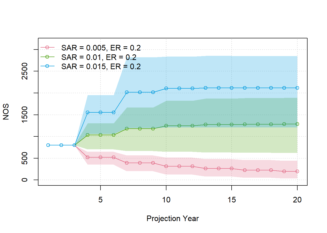
We can visualize the distribution of outcomes within scenarios with
compare_statevar_hist(), which has choices to plot with
either the density() or hist() functions:
compare_statevar_hist(SMSE_list[1:3], var = "NOS", names = SMSE_names[1:3], type = "density")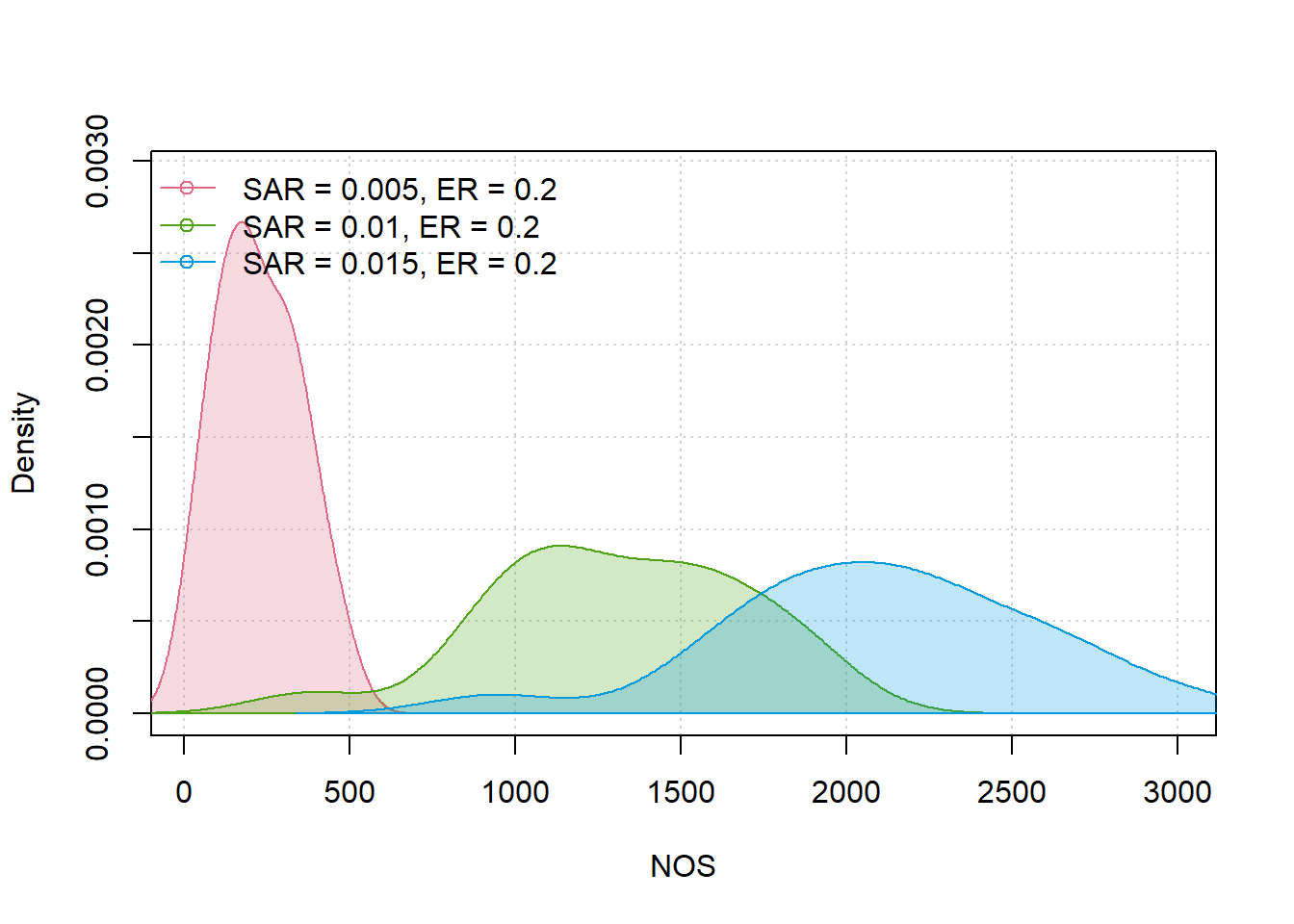
compare_statevar_hist(SMSE_list[1:3], var = "NOS", names = SMSE_names[1:3], type = "hist")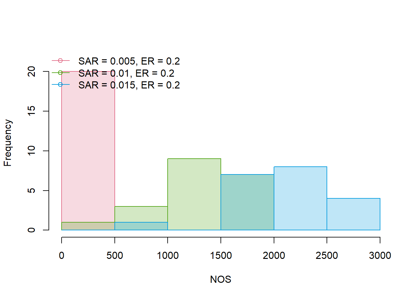
Performance measures and decision tables
Risk evaluation typically entails calculating a summary metric that describes the frequency that an objective was met in the simulation.
For example, we can calculate the probability that spawner abundance
exceeded 0.85 SMSY (spawners at MSY). We have a function
SMSY85() that does the calculation for us:
Using the vectorization capabilities in R, we use
sapply() to call SMSY85() for each of the
objects in SMSE_list. We add an extra argument
Yrs = c(20, 20) that specify the year range (the
probability is calculated at the end of the projection in year 20):
sim_results <- simulation_design
sim_results$spawner_objective <- sapply(SMSE_list, SMSY85, Yrs = c(20, 20))
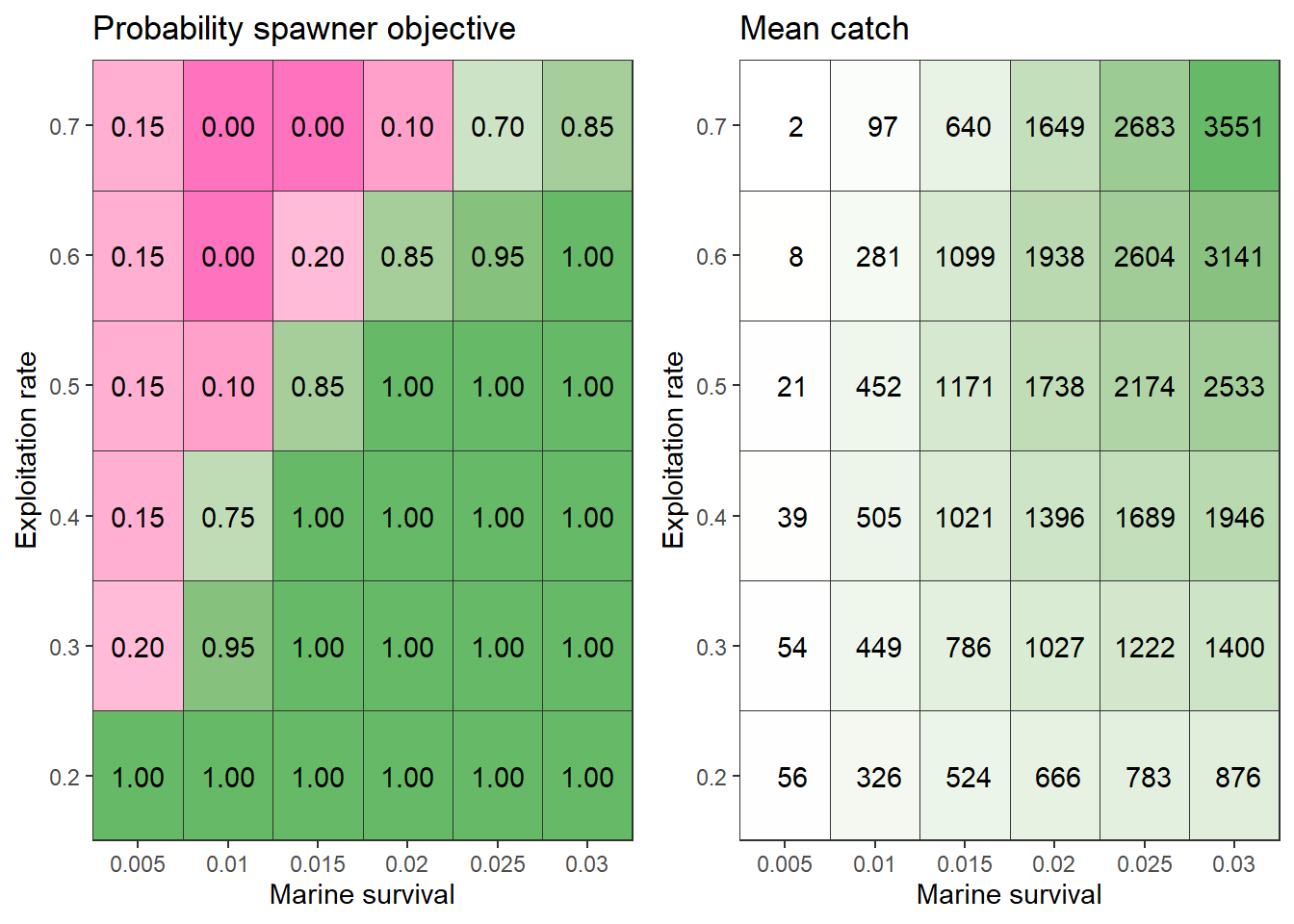
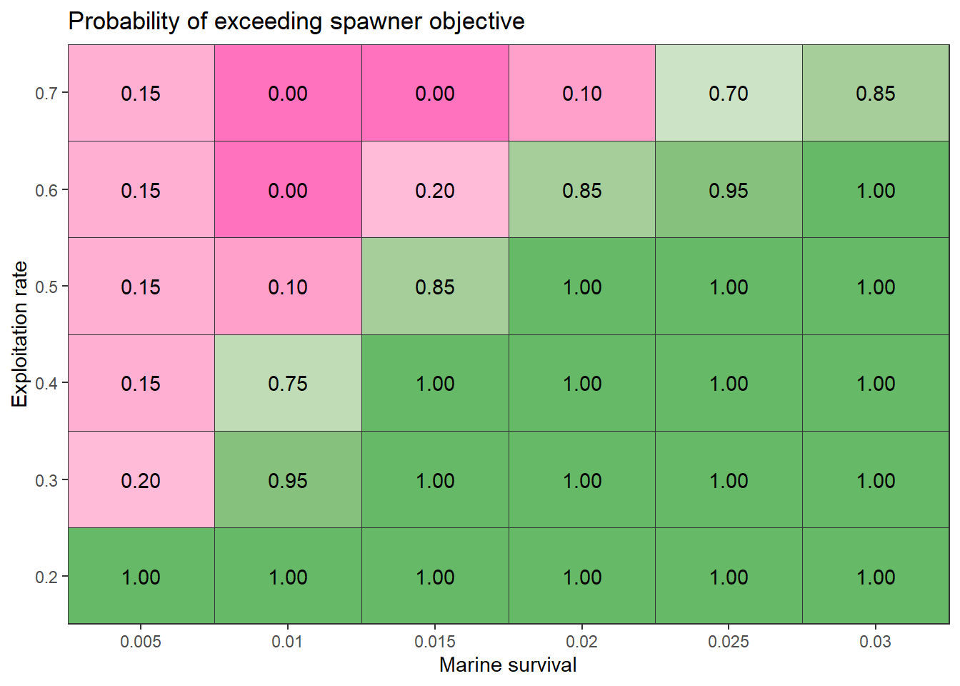
We want to explore the decision space: at what exploitation rates are we likely to reach our objective across plausible values of marine survival?
plot_decision_table() helps us plot a grid of values
using ggplot. The colour scheme maps 0-1 with red to green (0.5 is
white).
We can see a nice frontier line that delineates our decision-making space: we can meet our spawner objective with higher exploitation rates only if marine survival increases as well. Exploitation rates of 0.2 would be most robust to the marine survival scenarios that we simulated.
We can envision running a larger grid to map out the full decision space.
plot_decision_table(
  x = sim_results$SAR_vector,
  y = sim_results$ER_vector,
  z = sim_results$spawner_objective,
  xlab = "Marine survival",
  ylab = "Exploitation rate",
  title = "Probability of exceeding spawner objective"
)
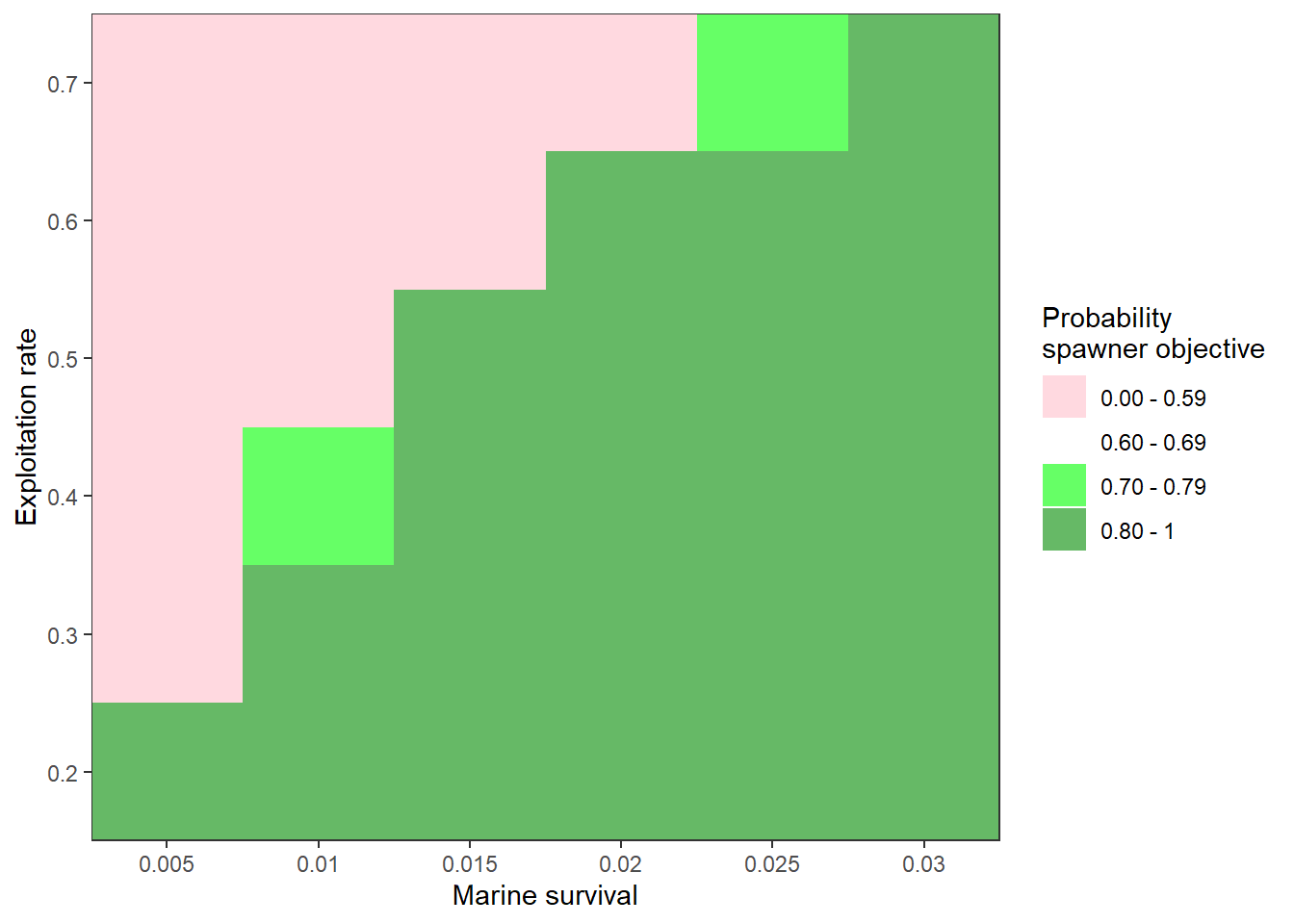
Alternatively, plot_decision_table2() gives us more
flexibility in the colour scheme by binning the summary metric into
separate colour bins. With the same layout as the previous figure, we
refine the decision table based on the outcomes:
plot_decision_table2(
  x = sim_results$SAR_vector,
  y = sim_results$ER_vector,
  z = sim_results$spawner_objective,
  xlab = "Marine survival",
  ylab = "Exploitation rate",
  zlab = "Probability\nspawner objective",
  bin = c(0, 0.6, 0.7, 0.8),
  bin_labels = c("0.00 - 0.59", "0.60 - 0.69", "0.70 - 0.79", "0.80 - 1"),
  bin_col = c("pink", "white", "green", "green4")
)
Tradeoffs
Frequently, objectives are conflicting. For example, lower exploitation rates in the long-run can allow for more escapement at the cost of catch. Tradeoff figures allow us to compare two summary metrics simultaneously.
First, let’s calculate our second metric, average catch in year 20, with a custom function:
Catch_fn <- function(SMSE) mean(rowSums(SMSE@KT_NOS[, 1, , 20])) # Kept catch of natural-origin fish
sim_results$Mean_catch <- sapply(SMSE_list, Catch_fn)
Next, we can use plot_tradeoff() to plot the two metrics
(average catch and spawner probability) against each other.
Typically, we want a nice frontier line that allows us to see the impact of our management options as in the decision tables above, but the tradeoff figure is quite messy:
plot_tradeoff(
  pm1 = sim_results$spawner_objective,
  pm2 = sim_results$Mean_catch,
  x1 = sim_results$ER_vector,
  x2 = sim_results$SAR_vector,
  xlab = "Probability spawner objective",
  ylab = "Mean catch",
  x1lab = "Exploitation rate",
  x2lab = "Marine survival"
)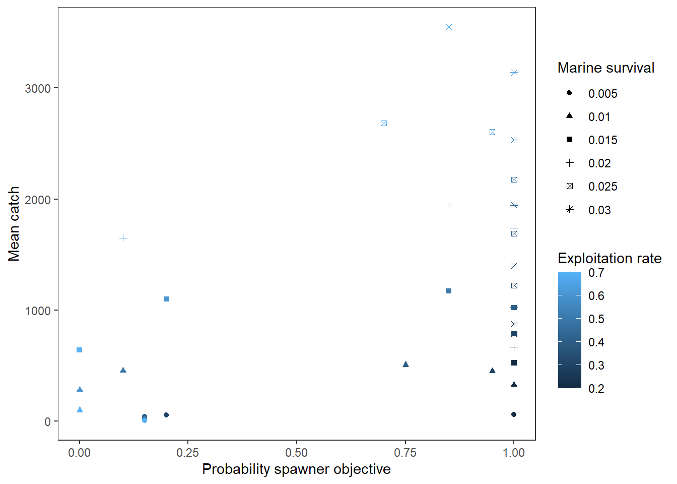
Tutorial 4 has an example with a more defined frontier in the tradeoff plot.
A sufficient alternative would be to plot the decision tables next to each other:
g1 <- plot_decision_table(
  x = sim_results$SAR_vector,
  y = sim_results$ER_vector,
  z = sim_results$spawner_objective,
  xlab = "Marine survival",
  ylab = "Exploitation rate",
  title = "Probability spawner objective"
)

g2 <- plot_decision_table(
  x = sim_results$SAR_vector,
  y = sim_results$ER_vector,
  z = round(sim_results$Mean_catch),
  xlab = "Marine survival",
  ylab = "Exploitation rate",
  title = "Mean catch"
)

cowplot::plot_grid(g1, g2)