salmonMSE utilizes an age-structured model in the projections. The population is tracked by age and year but various dynamics correspond to the salmon life stages as described below.
The model is also stochastic, for example, biological parameters representing uncertainty in the state of nature can be drawn from a probability distribution. For simplicity, the equations here describe the dynamics in a single simulation run. Potential stochastic parameters are noted in the package documentation.
1 Variable definitions
Definition of variable names and the corresponding slots in either the input (SOM) or output (SMSE) objects in salmonMSE.
1.1 Natural production
| Name | Definition | Type | Class | Slot |
|---|---|---|---|---|
| \(\textrm{NOS}\) | Natural origin spawners | Natural production | SMSE | NOS |
| \(\textrm{Fry}^\textrm{NOS}\) | Fry production by natural origin spawners | Natural production | SMSE | Fry_NOS |
| \(\textrm{Smolt}^\textrm{NOS}\) | Smolt production by natural origin spawners | Natural production | SMSE | Smolt_NOS |
| \(C_\textrm{egg-smolt}\) | Carrying capacity of smolts (Beverton-Holt stock-recruit parameter) | Natural production | SOM, Bio | capacity |
| \(S_\textrm{max}\) | Spawner abundance that maximizes smolt production (Ricker stock-recruit parameter) | Natural production | SOM, Bio | Smax |
| \(\kappa\) | Productivity (maximum recruitment production rate), units of recruit per spawner | Natural production | SOM, Bio | kappa |
| \(\phi\) | Unfished per capita egg production rate, units of egg per smolt | Natural production | SOM, Bio | phi |
| \(\tau\) | Unfished per capita spawners, units of spawner per smolt | Natural production | SOM, Bio | tau |
| \(r\) | Maturity at age, i.e., recruitment rate | Natural production | SOM, Bio | p_mature |
| \(\textrm{Fec}\) | Fecundity of spawners (eggs per female) | Natural production | SOM, Bio | fec |
| \(p^\textrm{female}\) | Proportion of female spawners in the natural environment | Natural production | SOM, Bio | p_female |
| \(\textrm{SAR}\) | Smolt-to-adult recruit survival | Natural production | - | - |
| \(M\) | Juvenile instantaneous natural mortality (marine environment) by origin | Natural production + Hatchery | SOM, Bio | Mjuv_NOS, Mjuv_HOS |
| \(s_\textrm{enroute}\) | Survival of escapement to spawning grounds and hatchery | Natural production | SOM, Bio | s_enroute |
| \(\textrm{NOR}\) | Natural origin return | Natural production | SMSE | Return_NOS |
1.2 Harvest
| Name | Definition | Type | Class | Slot |
|---|---|---|---|---|
| \(u^\textrm{PT}\) | Pre-terminal fishery harvest rate (adjusted for adult equivalents) | Harvest | SOM | u_preterminal |
| \(u^\textrm{T}\) | Terminal fishery harvest rate | Harvest | SOM | u_terminal |
| \(\delta\) | Mortality from catch and release (proportion) | Harvest | SOM | release_mort |
| \(v\) | Relative vulnerability by age to the fishery | Harvest | SOM | vulPT, vulT |
1.3 Hatchery
| Name | Definition | Type | Class | Slot |
|---|---|---|---|---|
| \(\textrm{HOS}\) | Hatchery origin spawners | Hatchery | SMSE | HOS |
| \(\textrm{HOS}_\textrm{eff}\) | Effective number of HOS, spawning output discounted by \(\gamma\) | Hatchery | SMSE | HOSeff |
| \(\textrm{Fry}^\textrm{HOS}\) | Fry production by hatchery origin spawners | Hatchery | SMSE | Fry_HOS |
| \(\textrm{Smolt}^\textrm{HOS}\) | Smolt production by hatchery origin spawners | Hatchery | SMSE | Smolt_HOS |
| \(\textrm{Fec}^\textrm{brood}\) | Fecundity of broodtake (eggs per female) | Hatchery | SOM, Hatchery | fec_brood |
| \(M\) | Juvenile instantaneous natural mortality (marine environment) by origin | Natural production + Hatchery | SOM, Bio | Mjuv_NOS, Mjuv_HOS |
| \(\textrm{NOB}\) | Natural origin broodtake | Hatchery | SMSE | NOB |
| \(\textrm{HOB}\) | Hatchery origin broodtake | Hatchery | SMSE | HOB |
| \(\textrm{Stray}\) | External strays of hatchery origin fish | Hatchery | SOM | stray_external |
| \(\textrm{HOB}_\textrm{stray}\) | Broodtake from strays | Hatchery | SMSE | HOB_stray |
| \(\textrm{Brood}^\textrm{avail,import}\) | Available imported brood (considered 100% marked) | Hatchery | SOM | brood_import |
| \(\textrm{Brood}^\textrm{import}\) | Realized imported fish used for brood (considered 100% marked) | Hatchery | SMSE | HOB_import |
| \(s_\textrm{yearling}\) | Survival of hatchery eggs to yearling life stage | Hatchery | SOM | s_egg_smolt |
| \(s_\textrm{subyearling}\) | Survival of hatchery eggs to subyearling life stage | Hatchery | SOM | s_egg_subyearling |
| \(p_\textrm{yearling}\) | Proportion of hatchery releases as yearling (vs. subyearling) | Hatchery | Internal state variable | - |
| \(s_\textrm{prespawn}\) | Survival of adult broodtake in hatchery | Hatchery | SOM | s_prespawn |
| \(n_\textrm{yearling}\) | Target number of hatchery releases as yearlings | Hatchery | SOM | n_yearling |
| \(n_\textrm{subyearling}\) | Target number of hatchery releases as subyearlings | Hatchery | SOM | n_subyearling |
| \(m\) | Mark rate of hatchery-origin fish | Hatchery | SOM | m |
| \(p^\textrm{esc}_\textrm{max}\) | Maximum proportion of total escapement (after en-route mortality) to use as broodtake | Hatchery | SOM | pmax_esc |
| \(p^\textrm{NOB}_\textrm{target}\) | Target proportion of broodtake that is natural origin, i.e., NOB/(NOB + HOB) ratio | Hatchery | SOM | ptarget_NOB |
| \(p^\textrm{NOB}_\textrm{max}\) | Maximum proportion of the natural origin broodtake from the escapement (after en-route mortality), i.e., NOB/NOS ratio | Hatchery | SOM | pmax_NOB |
| \(p_\textrm{NOB}\) | Realized proportion of brood that is natural-origin | Hatchery | SMSE | pNOB |
| \(\textrm{HOR}\) | Hatchery origin return | Hatchery | SMSE | Return_HOS |
| \(p^\textrm{hatchery}\) | Proportion of hatchery origin escapement returning to hatchery, available for broodtake | Hatchery | SOM | phatchery |
| \(p^\textrm{HOS}_\textrm{removal}\) | Proportion of hatchery origin fish removed from spawning grounds, not available for broodtake | Hatchery | SOM | premove_HOS |
| \(p^\textrm{NOS}_\textrm{removal}\) | Proportion of natural origin fish removed from spawning grounds, not available for broodtake | Hatchery | SOM | premove_NOS |
| \(\gamma\) | Reduced reproductive success of HOS | Hatchery | SOM | gamma |
| \(\bar{z}\) | Mean phenotypic value of cohort in natural and hatchery environments | Fitness | Internal state variable and SOM | zbar_start |
| \(\theta\) | Optimal phenotypic value for natural and hatchery environments | Fitness | SOM | theta |
| \(\sigma^2\) | Variance of phenotypic traits in population | Fitness | SOM | phenotype_variance |
| \(\omega^2\) | Variance of fitness function | Fitness | SOM | fitness_variance |
| \(h^2\) | Heritability of phenotypic traits | Fitness | SOM | heritability |
| \(\bar{W}\) | Population fitness in the natural and hatchery environments | Fitness | SMSE | fitness |
| \(\ell_i\) | Relative fitness loss at the life stage i (egg, fry, smolt) | Fitness | SOM | rel_loss |
| \(\textrm{PNI}\) | Proportionate natural influence | Fitness | SMSE | PNI |
| \(p_\textrm{HOSeff}\) | Proportion of effective hatchery origin spawners (vs. NOS) | Hatchery | SMSE | pHOS_effective |
| \(p_\textrm{HOScensus}\) | Proportion of hatchery origin spawners (vs. NOS) | Hatchery | SMSE | pHOS_census |
| \(p^\textrm{WILD}\) | Proportion of wild spawners | Hatchery | SMSE | p_wild |
1.4 Habitat
| Name | Definition | Type | Class | Slot |
|---|---|---|---|---|
| \(P^\textrm{ps}\) | Productivity for density-dependent survival: pre-spawn mortality | Habitat | SOM | prespawn_prod |
| \(C^\textrm{ps}\) | Capacity for density-dependent survival: pre-spawn mortality | Habitat | SOM | prespawn_capacity |
| \(P^\textrm{inc}\) | Productivity for density-dependent survival: egg incubation from spawning output | Habitat | SOM | egg_prod |
| \(C^\textrm{inc}\) | Capacity for density-dependent survival: egg incubation from spawning output | Habitat | SOM | egg_capacity |
| \(P^\textrm{egg-fry}\) | Productivity for density-dependent survival: egg emergence to fry life stage | Habitat | SOM | fry_prod |
| \(C^\textrm{egg-fry}\) | Capacity for density-dependent survival: egg emergence to fry life stage | Habitat | SOM | fry_capacity |
| \(\varepsilon^\textrm{egg-fry}_y\) | Deviations in density-dependent survival: egg to fry life stage | Habitat | SOM | fry_sdev |
| \(P^\textrm{fry-smolt}\) | Productivity for density-dependent survival: fry to smolt life stage | Habitat | SOM | smolt_prod |
| \(C^\textrm{fry-smolt}\) | Capacity for density-dependent survival: fry to smolt life stage | Habitat | SOM | smolt_capacity |
| \(\varepsilon^\textrm{fry-smolt}_y\) | Deviations in density-dependent survival: fry to smolt life stage | Habitat | SOM | smolt_sdev |
2 Juvenile natural production
First, we consider natural production in the absence of fitness effects arising from hatchery production.
The outmigrating juveniles of the next generation is predicted from the spawners from the previous year. Two parameterizations are possible:
- No habitat modeling: juvenile production is predicted from the egg production with a single density-dependent function
- With habitat modeling: juvenile production is predicted from a series of density-dependent functions that represent survival at intermittent freshwater life stages
2.1 No habitat modeling
From the spawners (NOS and HOS) of age \(a\) in year \(y\), the corresponding spawning output (units of eggs) of the subsequent generation is calculated as:
\[\begin{align} \textrm{Egg}^\textrm{NOS}_y &= \sum_a\textrm{NOS}_{y,a} \times p^\textrm{female}_a \times \textrm{Fec}_a\\ \textrm{Egg}^\textrm{HOS}_y &= \sum_a\textrm{HOS}_{\textrm{eff}y,a} \times p^\textrm{female}_a \times \textrm{Fec}_a \end{align}\]
where \(\textrm{HOS}_{\textrm{eff}} = \gamma \times \textrm{HOS}\) and the superscript denotes the parentage of the progeny.
In the output, fry production is assumed to be equal to spawning output, i.e., \(\textrm{Fry}^\textrm{NOS}_{y+1} = \textrm{Egg}^\textrm{NOS}_y\) and \(\textrm{Fry}^\textrm{HOS}_{y+1} = \textrm{Egg}^\textrm{HOS}_y\).
If the smolt production is calculated from the Ricker stock-recruit relationship, effectively over the entire freshwater life stage:
\[\begin{align} \textrm{Smolt}^\textrm{NOS}_{y+1} &= \alpha \times \textrm{Egg}^\textrm{NOS}_y\times\exp(-\beta[\textrm{Egg}^\textrm{NOS}_y + \textrm{Egg}^\textrm{HOS}_y])\\ \textrm{Smolt}^\textrm{HOS}_{y+1} &= \alpha \times \textrm{Egg}^\textrm{HOS}_y\times\exp(-\beta[\textrm{Egg}^\textrm{NOS}_y + \textrm{Egg}^\textrm{HOS}_y]) \end{align}\]
where:
\[\begin{align} \alpha &= \kappa/\phi\\ \beta &= 1/{E_\textrm{max}}\\ E_\textrm{max} &= S_\textrm{max} \times \phi/\tau\\ \phi &= \sum_a\left(\prod_{i=1}^{a-1}\exp(-M^\textrm{NOS}_i)(1-r_i)\right)\times r_a \times p^\textrm{female}_a \times \textrm{Fec}_a\\ \tau &= \sum_a\left(\prod_{i=1}^{a-1}\exp(-M^\textrm{NOS}_i)(1-r_i)\right)\times r_a \times p^\textrm{female}_a \end{align}\]
\(\kappa\) is the productivity, \(\phi\) is the egg production per smolt at replacement, and \(\tau\) is the female spawner per smolt at replacement.
With the Beverton-Holt stock-recruit relationship, the age-1 smolt production is
\[\begin{align} \textrm{Smolt}^\textrm{NOS}_{y+1} &= \frac{\alpha \times \textrm{Egg}^\textrm{NOS}_y}{1 + \beta(\textrm{Egg}^\textrm{NOS}_y + >\textrm{Egg}^\textrm{HOS}_y)}\\ \textrm{Smolt}^\textrm{HOS}_{y+1} &= \frac{\alpha \times \textrm{Egg}^\textrm{HOS}_y}{1 + \beta(\textrm{Egg}^\textrm{NOS}_y + >\textrm{Egg}^\textrm{HOS}_y)} \end{align}\]
where \(\alpha = \kappa/\phi\), \(\beta = \alpha/{C_\textrm{egg-smolt}}\) (\(C\) is the capacity/asymptote).
The density-independent component of the survival equation is controlled by \(\alpha\) and the density-dependent component of survival is controlled by \(\beta\) and scaled by the total egg production (see Hatchery section).
2.2 With habitat modeling
Freshwater life stages can also be modeled as a series of density-dependent functions by life stage, following the general approach of Jorgensen et al. 2021. Four relationships are modeled:
- Pre-spawn mortality
- Egg incubation mortality
- Egg emergence to fry mortality
- Fry to smolt mortality
Survival is modeled through either a Beverton-Holt or hockey-stick function that predicts survivors from the abundance at the beginning of the life stage.
Example life stage density-dependent relationships. Left panel: Beverton-Holt function. Right panel: Hockey-stick function. For both panels, the productivity is 0.8 and capacity is 600.
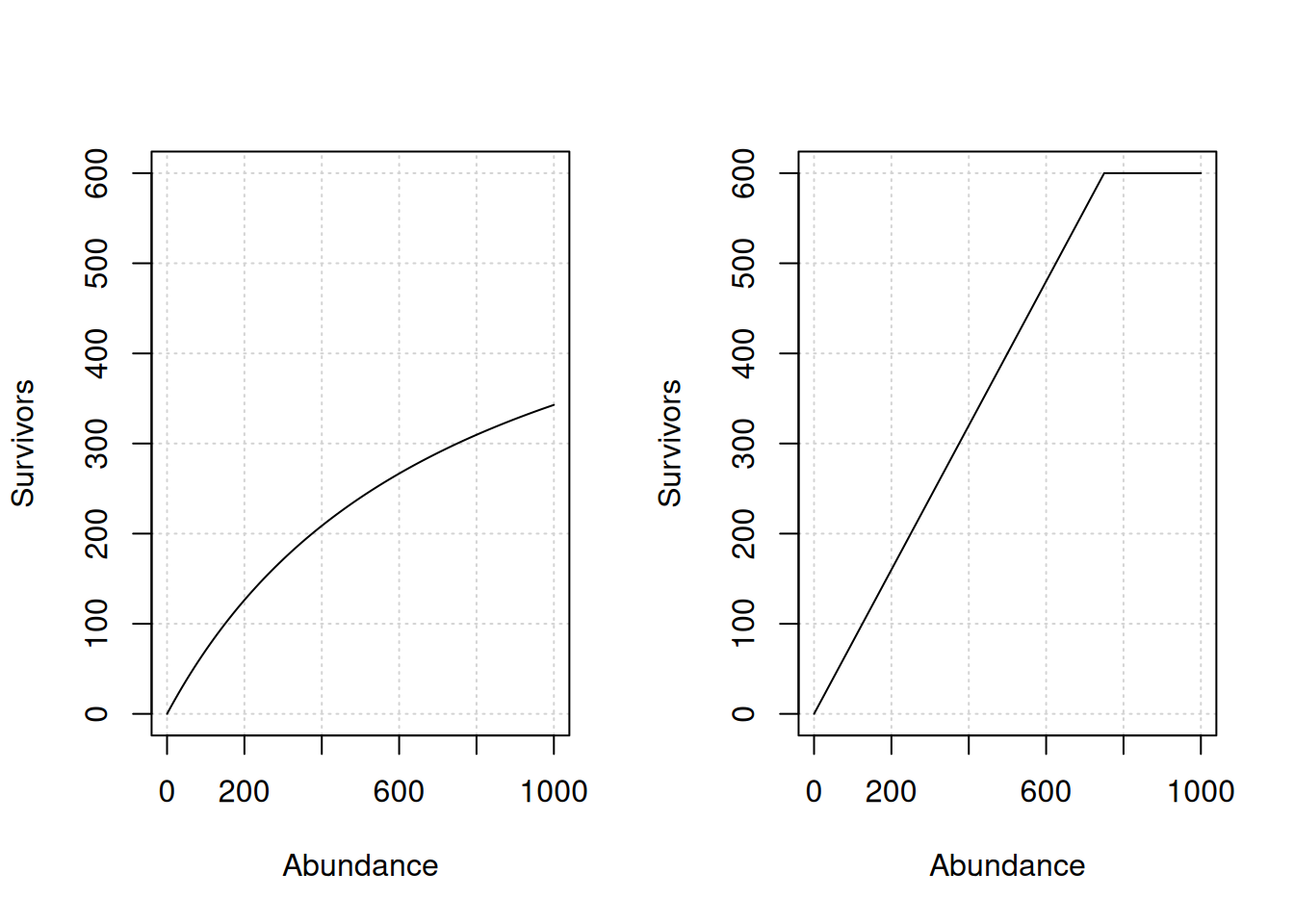
Set the capacity to infinite to model density-independence. The productivity parameter is then the survival to the next life stage.
First, pre-spawn (ps) mortality can occur, where the surviving spawners \(\widetilde{\textrm{NOS}}_y\) and \(\widetilde{\textrm{HOS}}_y\) are:
\[\begin{align} \widetilde{\textrm{NOS}}_y &= \frac{P^\textrm{ps} \times \textrm{NOS}_y}{1 + \frac{P^\textrm{ps}}{C^\textrm{ps}}(\textrm{NOS}_y + \textrm{HOS}_y)}\\ \widetilde{\textrm{HOS}}_y &= \frac{P^\textrm{ps} \times \textrm{HOS}_y}{1 + \frac{P^\textrm{ps}}{C^\textrm{ps}}(\textrm{NOS}_y + \textrm{HOS}_y)}\\ \end{align}\]
where productivity \(P\) is the maximum survival as spawner numbers approaches zero and \(C\) is the asymptotic number of spawners, i.e., spawner capacity.
The hockey-stick equation is
\[\begin{align} \widetilde{\textrm{NOS}}_y &= \textrm{min}(P^\textrm{ps} \times \textrm{NOS}_y, (\frac{\textrm{NOS}_y}{\textrm{NOS}_y + \textrm{HOS}_y}) C^\textrm{ps})\\ \widetilde{\textrm{HOS}}_y &= \textrm{min}(P^\textrm{ps} \times \textrm{HOS}_y, (\frac{\textrm{HOS}_y}{\textrm{NOS}_y + \textrm{HOS}_y}) C^\textrm{ps}) \end{align}\]
with similar parameterizations for subsequent life stages (not further described below).
The initial egg production is calculated after pre-spawn mortality:
\[\begin{align} \textrm{Egg}^\textrm{NOS}_y &= \sum_a\widetilde{\textrm{NOS}}_{y,a} \times p^\textrm{female}_a \times \textrm{Fec}_a\\ \textrm{Egg}^\textrm{HOS}_y &= \sum_a\widetilde{\textrm{HOS}}_{\textrm{eff}y,a} \times p^\textrm{female}_a \times \textrm{Fec}_a \end{align}\]
Second, the surviving egg production (\(\widetilde{\textrm{Egg}}_y\)) can be reduced from the initial spawning output (\(\textrm{Egg}_y\)) due to incubation mortality. With a Beverton-Holt function:
\[\begin{align} \widetilde{\textrm{Egg}}^\textrm{NOS}_y &= \frac{P^\textrm{inc} \times \textrm{Egg}^\textrm{NOS}_y}{1 + \frac{P^\textrm{inc}}{C^\textrm{inc}}(\textrm{Egg}^\textrm{NOS}_y + \textrm{Egg}^\textrm{HOS}_y)}\\ \widetilde{\textrm{Egg}}^\textrm{HOS}_y &= \frac{P^\textrm{inc} \times \textrm{Egg}^\textrm{HOS}_y}{1 + \frac{P^\textrm{inc}}{C^\textrm{inc}}(\textrm{Egg}^\textrm{NOS}_y + \textrm{Egg}^\textrm{HOS}_y)} \end{align}\]
where productivity \(P\) is the maximum survival as spawning output approaches zero and \(C\) is the asymptotic production (egg capacity).
Third, fry production is modeled as:
\[\begin{align} \textrm{Fry}^\textrm{NOS}_{y+1} &= \frac{P^\textrm{egg-fry} \times \widetilde{\textrm{Egg}}^\textrm{NOS}_y}{1 + \frac{P^\textrm{egg-fry}}{C^\textrm{egg-fry}}(\widetilde{\textrm{Egg}}^\textrm{NOS}_y + \widetilde{\textrm{Egg}}^\textrm{HOS}_y)} \times \varepsilon^\textrm{egg-fry}_y\\ \textrm{Fry}^\textrm{HOS}_{y+1} &= \frac{P^\textrm{egg-fry} \times \widetilde{\textrm{Egg}}^\textrm{HOS}_y}{1 + \frac{P^\textrm{egg-fry}}{C^\textrm{egg-fry}}(\widetilde{\textrm{Egg}}^\textrm{NOS}_y + \widetilde{\textrm{Egg}}^\textrm{HOS}_y)} \times \varepsilon^\textrm{egg-fry}_y \end{align}\]
where \(\varepsilon^\textrm{egg-fry}_y\) is a year-specific deviation in survival. They can be modeled as a function of a proposed time series of environmental variables \(\eta\), for example, \(\varepsilon^\textrm{egg-fry}_y = \prod_j f(\eta_{y,j})\) or \(\varepsilon^\textrm{egg-fry}_y = \sum_j f(\eta_{y,j})\).
The last freshwater life stage with smolt production is modeled as:
\[\begin{align} \textrm{Smolt}^\textrm{NOS}_y &= \frac{P^\textrm{fry-smolt} \times \textrm{Fry}^\textrm{NOS}_y}{1 + \frac{P^\textrm{fry-smolt}}{C^\textrm{fry-smolt}}(\textrm{Fry}^\textrm{NOS}_y + \textrm{Fry}^\textrm{HOS}_y)} \times \varepsilon^\textrm{fry-smolt}_y\\ \textrm{Smolt}^\textrm{HOS}_y &= \frac{P^\textrm{fry-smolt} \times \textrm{Fry}^\textrm{HOS}_y}{1 + \frac{P^\textrm{fry-smolt}}{C^\textrm{fry-smolt}}(\textrm{Fry}^\textrm{NOS}_y + \textrm{Fry}^\textrm{HOS}_y)} \times \varepsilon^\textrm{fry-smolt}_y \end{align}\]
Alternative scenarios with changes in productivity or capacity parameters can be used to evaluate changes in life stage survival from habitat improvement or mitigation measures as part of a management strategy, or from climate regimes (low productivity vs. high productivity, or low capacity vs. high capacity). An increase in capacity can arise from restoration which increases the area of suitable habitat. An increase in productivity can arise from improvement in habitat, e.g., sediment quality. Year-specific deviations can be used to simulate stochasticity in survival.
Approaches such as HARP and CEMPRA can inform productivity and capacity parameters across these life stages as quantitative relationships between habitat variables.
2.3 Competition with hatchery releases
Competition between natural-origin fish and hatchery releases can be incorporated into the density-dependent survival equation by adjusting the denominator of the Beverton-Holt equation:
\[\begin{align} \textrm{Smolt}^\textrm{NOS}_y &= \frac{P^\textrm{fry-smolt} \times \textrm{Fry}^\textrm{NOS}_y}{1 + \frac{P^\textrm{fry-smolt}}{C^\textrm{fry-smolt}}(\textrm{Fry}^\textrm{NOS}_y + \textrm{Fry}^\textrm{HOS}_y + n^\textrm{subyearling}_y + n^\textrm{yearling}_y)} \times \varepsilon^\textrm{fry-smolt}_y\\ \textrm{Smolt}^\textrm{HOS}_y &= \frac{P^\textrm{fry-smolt} \times \textrm{Fry}^\textrm{HOS}_y}{1 + \frac{P^\textrm{fry-smolt}}{C^\textrm{fry-smolt}}(\textrm{Fry}^\textrm{NOS}_y + \textrm{Fry}^\textrm{HOS}_y + n^\textrm{subyearling}_y + n^\textrm{yearling}_y)} \times \varepsilon^\textrm{fry-smolt}_y \end{align}\]
where \(n^\textrm{subyearling}_y\) and \(n^\textrm{yearling}_y\) are subyearling and yearling releases from the hatchery, respectively.
salmonMSE can be modified so that either subyearling, yearling, or both types of releases are included in the density-dependence term. This competition could be modeled for stream-type life histories.
3 Hatchery juvenile production
Hatchery production is controlled by several parameters specified by the analyst, roughly following the AHA approach. The three main parameters are to:
- Specify target releases
- Specify target proportion natural-origin fish in the brood
- Specify limit proportion of natural-origin return to use as brood
The first parameter specifies the target number of annual releases of sub-yearlings \(n^\textrm{subyearling}_\textrm{target}\) and yearlings \(n^\textrm{yearling}_\textrm{target}\). For the purposes of hatchery releases, yearlings and subyearlings are only differentiated by egg to release survival in the hatchery, for example, yearlings have lower egg-release survival if they are released later.
Going backwards, the corresponding number of eggs needed to reach the target number depends on the egg survival to those life stages in the hatchery. The corresponding number of broodtake is calculated from target egg production based on the brood fecundity and hatchery survival of broodtake, which is non-selective with respect to age.
The second parameter is the target proportion of natural-origin fish in the broodstock \(p^\textrm{NOB}_\textrm{target}\). To minimize genetic drift of the population due to hatchery production, it may be desirable to maintain a high proportion of natural-origin broodtake.
This target is possible if the mark rate is one (one can identify all hatchery-origin fish in the in-river return). If the mark rate is not 1, then \(p^\textrm{NOB}_\textrm{target}\) is the target proportion of unmarked fish in the broodtake. Consequently, the realized \(p^\textrm{NOB}\) is reduced as some of the unmarked fish are hatchery-origin.
The target also may not be met in cases with low returns and brood is continually taken to meet the release target.
The third parameter is \(p^\textrm{NOB}_\textrm{max}\), the maximum allowable proportion of the natural-origin return to be used as broodtake. This value is never exceeded.
To set up a segregated hatchery program, set \(p^\textrm{NOB}_\textrm{max} = 0\). Otherwise, these equations set up an integrated hatchery.
The following equations generate the annual broodtake and hatchery production from the state variables given constraints from these parameters.
3.1 Broodtake
The annual target egg production for the hatchery is calculated from the target releases as
\[ \textrm{Egg}_\textrm{target,broodtake} = \dfrac{n^\textrm{yearling}_\textrm{target}}{s^\textrm{yearling}} + \dfrac{n^\textrm{subyearling}_\textrm{target}}{s^\textrm{subyearling}} \]
where \(s\) is survival from the egg to the corresponding life stage in the hatchery.
The broodtake is back-calculated from the target egg production. From annual escapement from marine fisheries (\(\textrm{NOR}^\textrm{escapement}\) and \(\textrm{HOR}^\textrm{escapement}\)), some proportion \(p^\textrm{broodtake}\) is used as brood.
Natural-origin brood is taken from fish in passage to spawning grounds:
\[ \textrm{NOB}_{y,a} = p^\textrm{broodtake,unmarked}_y \times \textrm{NOR}^\textrm{avail,brood}_{y,a} \]
where \(\textrm{NOR}^\textrm{avail,brood}_{y,a} = \textrm{NOR}^\textrm{escapement} \times s_\textrm{enroute} \times p^\textrm{esc}_\textrm{max}\) is the available fish for brood, reduced by en-route mortality (with survival \(s_\textrm{enroute}\)), and limited some proportion denoted by the \(p^\textrm{esc}_\textrm{max}\) parameter.
Hatchery-origin brood could be taken in two ways:
- From fish “returning to the hatchery”, e.g., through swim-in facilities or removal from spawning grounds:
\[\begin{align} \textrm{HOB}^\textrm{unmarked}_{y,a} &= p^\textrm{broodtake,unmarked}_y \times (1-m) \times \textrm{HOR}^\textrm{avail,brood}_{y,a}\\ \textrm{HOB}^\textrm{marked}_{y,a} &= p^\textrm{broodtake,marked}_y \times m \times \textrm{HOR}^\textrm{avail,brood}_{y,a} \end{align}\]
where \(\textrm{HOR}^\textrm{avail,brood}_{y,a} = p^\textrm{hatchery} \times \textrm{HOR}^\textrm{escapement}_{y,a} \times s_\textrm{enroute} \times p^\textrm{esc}_\textrm{max}\) and \(p^\textrm{hatchery}\) is the proportion returning to the hatchery.
- From fish in passage to spawning grounds, same as case #1 but with \(\textrm{HOR}^\textrm{avail,brood}_{y,a} = \textrm{HOR}^\textrm{escapement}_{y,a} \times s_\textrm{enroute} \times p^\textrm{esc}_\textrm{max}\)
Imported brood and strays may also be used:
\[\begin{align} \textrm{Brood}^\textrm{import}_{y,a} &= p^\textrm{broodtake,marked}_y \sum_a \textrm{Brood}^\textrm{avail,import}_a\\ \textrm{HOB}^\textrm{stray}_{y,a} &= p^\textrm{broodtake,unmarked}_y \times \textrm{Stray}_{y,a} \times s_\textrm{enroute} \times p^\textrm{esc}_\textrm{max} \end{align}\]
To exclusively use imported brood, set \(p^\textrm{esc}_\textrm{max} = 0\).
The realized hatchery egg production is
\[\begin{align} \textrm{Egg}_\textrm{y}^\textrm{NOB} &= \sum_a \textrm{NOB}_{y,a} \times s^\textrm{prespawn} \times p^\textrm{female,brood}_a \times \textrm{Fec}^\textrm{brood}_a\\ \textrm{Egg}_\textrm{y}^\textrm{HOB} &= \sum_a (\textrm{HOB}^\textrm{marked}_{y,a} + \textrm{HOB}^\textrm{unmarked}_{y,a}) \times s^\textrm{prespawn} \times p^\textrm{female,brood}_a \times \textrm{Fec}^\textrm{brood}_a\\ \textrm{Egg}_\textrm{y}^\textrm{import} &= \sum_a \textrm{Brood}^\textrm{import}_{y,a} \times s^\textrm{prespawn} \times p^\textrm{female,brood}_a \times \textrm{Fec}^\textrm{brood}_a\\ \textrm{Egg}_\textrm{y}^\textrm{stray} &= \sum_a \textrm{HOB}^\textrm{stray}_{y,a} \times s^\textrm{prespawn} \times p^\textrm{female,brood}_a \times \textrm{Fec}^\textrm{brood}_a \end{align}\]
where broodstock is subject to a survival term \(s^\textrm{prespawn}\) prior to egg production.
The proportion \(p^\textrm{broodtake}_y\) is solved annually to satisfy the following conditions:
\(\dfrac{\sum_a(\textrm{NOB}_{y,a} + \textrm{HOB}^\textrm{unmarked}_{y,a} + \textrm{HOB}^\textrm{stray}_{y,a})}{\sum_a(\textrm{NOB}_{y,a} + \textrm{HOB}^\textrm{unmarked}_{y,a} + \textrm{HOB}^\textrm{marked}_{y,a} + \textrm{HOB}^\textrm{stray}_{y,a} + \textrm{Brood}^\textrm{import}_{y,a})} = p^\textrm{NOB}_\textrm{target}\)
\(0 < p^\textrm{broodtake,marked}_y \le 1\)
\(0 < p^\textrm{broodtake,unmarked}_y \le p^\textrm{NOB}_\textrm{max}\)
\(\textrm{Egg}_\textrm{y}^\textrm{NOB} + \textrm{Egg}_\textrm{y}^\textrm{HOB} + \textrm{Egg}_\textrm{y}^\textrm{import} + \textrm{Egg}^\textrm{stray}_y = \textrm{Egg}_\textrm{broodtake}\)
Total egg production in a given year can fail to reach the target if there is insufficient unmarked escapement and \(p^\textrm{broodtake,unmarked}_y = p^\textrm{NOB}_\textrm{max}\). In this case, the remaining deficit in egg production is met by increasing HOB (the realized \(p^\textrm{NOB}\) can be lower than the target).
3.1.1 Custom brood rule
A custom brood rule \(f\) is possible where the user specifies the brood taken from the available in-river return:
\[ \begin{pmatrix} \textrm{NOB}_{y,a}\\ \textrm{HOB}^\textrm{unmarked}_{y,a}\\ \textrm{HOB}^\textrm{marked}_{y,a}\\ \textrm{HOB}^\textrm{stray}_{y,a} \end{pmatrix} = f\!\left( \begin{matrix} \textrm{NOR}^\textrm{avail,brood}_{y,a}\\ \textrm{HOR}^\textrm{avail,brood}_{y,a}\\ \textrm{Stray}_{y,a}\\ m \end{matrix} \right) \]
3.2 Releases
After the total hatchery egg production is calculated, the production of yearlings and subyearlings is calculated to ensure the annual ratio is equal to the target ratio. To do so, the parameter \(p^\textrm{egg,yearling}_y\) is solved subject to the following conditions:
\(\textrm{Egg}_\textrm{brood,y} = \textrm{Egg}_\textrm{y}^\textrm{NOB} + \textrm{Egg}_\textrm{y}^\textrm{HOB} + \textrm{Egg}^\textrm{import}_y + \textrm{Egg}^\textrm{stray}_y\)
\(n^\textrm{yearling}_{y+1} = p^\textrm{egg,yearling}_y \times \textrm{Egg}_\textrm{brood,y} \times s^\textrm{yearling}\)
\(n^\textrm{subyearling}_{y+1} = (1 - p^\textrm{egg,yearling}_y) \times \textrm{Egg}_\textrm{brood,y} \times s^\textrm{subyearling}\)
\(\frac{n^\textrm{yearling}_y}{n^\textrm{subyearling}_y + n^\textrm{yearling}_y} = \frac{n^\textrm{yearling}_\textrm{target}}{n^\textrm{subyearling}_\textrm{target} + n^\textrm{yearling}_\textrm{target}}\)
With no density-dependent competition with natural-origin juveniles, the outmigrating releases (“smolt releases”) is calculated as
\[ \textrm{Smolt}^\textrm{Rel}_{y+1} = n^\textrm{subyearling}_{y+1} + n^\textrm{yearling}_{y+1} \]
With competition, the outmigrating abundance is:
\[ \textrm{Smolt}^\textrm{Rel}_{y+1} = \alpha \times (n^\textrm{subyearling}_{y+1} + n^\textrm{yearling}_{y+1}) \times \exp(-\beta(\textrm{Fry}^\textrm{NOS}_{y+1} + \textrm{Fry}^\textrm{HOS}_{y+1} + n^\textrm{subyearling}_{y+1} + n^\textrm{yearling}_{y+1})) \]
or
\[ \textrm{Smolt}^\textrm{Rel}_{y+1} = \frac{\alpha \times (n^\textrm{subyearling}_{y+1} + n^\textrm{yearling}_{y+1})}{1 + \beta(\textrm{Fry}^\textrm{NOS}_{y+1} + \textrm{Fry}^\textrm{HOS}_{y+1} + n^\textrm{subyearling}_{y+1} + n^\textrm{yearling}_{y+1})} \]
4 Juvenile marine abundance
Let \(N^\textrm{juv}_{y,a}\) be the juvenile abundance in the population at the beginning of the year, with \(N^\textrm{juv,NOS}_{y,a=1} = \textrm{Smolt}^\textrm{NOS}_y + \textrm{Smolt}^\textrm{HOS}_y\) and \(N^\textrm{juv,HOS}_{y,a=1} = \textrm{Smolt}^\textrm{Rel}\). The superscript for the smolt variable corresponds to the parentage while the superscript for \(N\) denotes the origin of the current cohort.
4.1 Pre-terminal fishery
Harvest \(u^\textrm{PT}\) in the pre-terminal (\(\textrm{PT}\)) fishery, ostensibly of juveniles, occurs in the first half of the year.
Assuming no mark-selective fishing, the kept catch \(K\) is
\[\begin{align} K^\textrm{NOS,PT}_{y,a} &= \left(1 - \exp(-v^\textrm{PT}_a F^\textrm{PT}_y)\right)N^\textrm{juv,NOS}_{y,a}\\ K^\textrm{HOS,PT}_{y,a} &= \left(1 - \exp(-v^\textrm{PT}_a F^\textrm{PT}_y)\right)N^\textrm{juv,HOS}_{y,a}\\ \end{align}\]
If management is by target harvest rate, then the specified harvest rate \(u^\textrm{PT}\) in the pre-terminal (\(\textrm{PT}\)) fishery is used to calculate \(F^\textrm{PT}_y\) such that:
\[ u^\textrm{PT}_y = \frac{\sum_a(K^\textrm{NOS,PT}_{y,a} + K^\textrm{HOS,PT}_{y,a})\times \textrm{AEQ}_a}{\sum_a\left((K^\textrm{NOS,PT}_{y,a} + K^\textrm{HOS,PT}_{y,a}) \times \textrm{AEQ}_a + (N^\textrm{juv,NOS}_{y,a} + N^\textrm{juv,HOS}_{y,a})\exp(-v^\textrm{PT}_a F^\textrm{PT}_y)\times r_a)\right)} \]
To facilitate comparison of juvenile catch to adult catch, adult equivalents (AEQ) discount the juvenile catch by how many would have survived to adulthood had it not been caught (through maturity and natural mortality):
\[ \textrm{AEQ}_a = \begin{cases} 1 &, a = A\\ r_a + (1 - r_a)\exp(-M_a) \times \textrm{AEQ}_{a+1} &, a = 1, \ldots, A-1 \end{cases} \]
If management is by target catch \(K^\textrm{PT,target}\), then \(F^\textrm{PT}_y\) is solved such that \(K^\textrm{PT,target} = \sum_a K^\textrm{NOS,PT}_{y,a} + \sum_a K^\textrm{HOS,PT}_{y,a}\).
Alternative equations are used if mark-selective fishing is implemented.
5 Recruitment and maturity
The recruitment is calculated from the survival of juvenile fish after pre-terminal harvest and maturation:
\[\begin{align} \textrm{NOR}_{y,a} &= N^\textrm{juv,NOS}_{y,a}\exp(-v_aF^\textrm{PT}_y)r_{y,a}\\ \textrm{HOR}_{y,a} &= N^\textrm{juv,HOS}_{y,a}\exp(-v_aF^\textrm{PT}_y)r_{y,a} \end{align}\]
5.1 Advance age classes
The juvenile abundance in the following year consists of fish that did not mature and subsequently survived natural mortality \(M\):
\[\begin{align} N^\textrm{juv,NOS}_{y+1,a+1} &= N^\textrm{juv,NOS}_{y,a}\exp\left(-[v_aF^\textrm{PT}_y + M^\textrm{NOS}_{y,a}]\right)(1 - r_{y,a})\\ N^\textrm{juv,HOS}_{y+1,a+1} &= N^\textrm{juv,HOS}_{y,a}\exp\left(-[v_aF^\textrm{PT}_y + M^\textrm{HOS}_{y,a}]\right)(1 - r_{y,a}) \end{align}\]
5.2 Terminal fishery
Assuming no mark-selective fishing, the kept catch of the terminal (\(\textrm{T}\)) fishery is calculated similarly as with the pre-terminal fishery:
\[\begin{align} K^\textrm{NOS,T}_{y,a} &= \left(1 - \exp(-v^\textrm{T}_a F^\textrm{T}_y)\right)\textrm{NOR}_{y,a}\\ K^\textrm{HOS,T}_{y,a} &= \left(1 - \exp(-v^\textrm{T}_a F^\textrm{T}_y)\right)\textrm{HOR}_{y,a}\\ \end{align}\]
If management is by target harvest rate, then the specified harvest rate \(u^\textrm{T}\) is used to calculate \(F^\textrm{T}\) such that
\[ u^\textrm{T}_y = \frac{\sum_a(K^\textrm{NOS,T}_{y,a} + K^\textrm{HOS,T}_{y,a})}{\sum_a(\textrm{NOR}_{y,a} + \textrm{HOR}_{y,a})} \]
If management is by target catch \(K^\textrm{T,target}\), then the fishing mortality is solved such that \(K^\textrm{T,target} = \sum_a K^\textrm{NOS,T}_{y,a} + \sum_a K^\textrm{HOS,T}_{y,a}\).
Alternative equations are used if mark-selective fishing is implemented.
6 Escapement and spawners
The escapement consists of the survivors of the terminal fishery:
\[\begin{align} \textrm{NOR}^\textrm{escapement}_{y,a} &= \textrm{NOR}_{y,a}\exp(-v_aF^\textrm{T}_y)\\ \textrm{HOR}^\textrm{escapement}_{y,a} &= \textrm{HOR}_{y,a}\exp(-v_aF^\textrm{T}_y) \end{align}\]
Natural-origin spawners is the escapement that survive return migration, are not used for brood, and are not removed from the spawning ground (e.g., as part of in-river fishery):
\[ \textrm{NOS}_{y,a} = (1 - p^\textrm{NOS}_\textrm{removal}\times(1-m))\left(\textrm{NOR}^\textrm{escapement}_{y,a} \times s_\textrm{enroute} - \textrm{NOB}_{y,a}\right) \]
If HOB are collected from fish returning to the hatchery, then the hatchery-origin spawners is:
\[\begin{align} \textrm{HOS}_{y,a} &= \textrm{HOS}^\textrm{local}_{y,a} + \textrm{HOS}^\textrm{stray}_{y,a}\\ &= (1 - p^\textrm{hatchery}) (1 - p^\textrm{HOS}_\textrm{removal} \times m) \textrm{HOR}^\textrm{escapement}_{y,a} \times s_\textrm{enroute} + (\textrm{Stray}_{y,a} \times s_\textrm{enroute} - \textrm{HOB}^\textrm{stray}_{y,a}) \end{align}\]
If HOB are collected from fish on the way to spawning grounds, then:
\[\begin{align} \textrm{HOS}_{y,a} &= \textrm{HOS}^\textrm{local}_{y,a} + \textrm{HOS}^\textrm{stray}_{y,a}\\ &= (1 - p^\textrm{HOS}_\textrm{removal} \times m) (\textrm{HOR}^\textrm{escapement}_{y,a} \times s_\textrm{enroute} - \textrm{HOB}_{y,a}) + (\textrm{Stray}_{y,a} \times s_\textrm{enroute} - \textrm{HOB}^\textrm{stray}_{y,a}) \end{align}\]
Hatchery-origin spawners is the escapement of local origin and strays that survive return migration, do not return to the hatchery (either by swim-in facilities or in-river collection), and are not removed from the spawning ground (through proportion \(p^\textrm{HOS}_\textrm{removal}\) and discounted by the mark rate, these animals are not available for brood). Strays not used for brood are also included as hatchery spawners.
7 Fitness effects on juvenile survival
Reproductive success of first generation hatchery fish has been observed to be lower than their natural counterparts, and is accounted for in the \(\gamma\) parameter (see review in Withler et al. 2018).
Through genetic and epigenetic factors, survival of hatchery juveniles in the hatchery environment selects for fish with a phenotype best adapted for that environment, and likewise for juveniles spawned in the natural environment. Since these traits are heritable, the fitness of the natural population can shift away from the optimum for the natural environment towards that of the hatchery environment on an evolutionary time scale, i.e., over a number of generations, when hatchery fish are allowed to spawn.
As described in Ford 2002 and derived in Lande 1976, the fitness loss function \(W\) for an individual with phenotypic trait value \(z\) in a given environment is
\[ W(z) = \exp\left(\dfrac{-(z-\theta)^2}{2\omega^2}\right) \]
where \(\theta\) is the optimum for that environment and \(\omega^2\) is the fitness variance.
If the phenotypic trait value \(z\) in the population is a random normal variable with mean \(\bar{z}\) and variance \(\sigma^2\), then the mean fitness of the population in generation \(g\) is \(\bar{W}(z) = \int W(z) f(z) dz\), where \(f(z)\) is the Gaussian probability density function. The solution is proportional to
\[ \bar{W}(z) \propto \exp\left(\dfrac{-(\bar{z}-\theta)^2}{2(\omega^2+\sigma^2)}\right) \]
The mean phenotype \(\bar{z}\) is calculated iteratively, where the change \(\Delta\bar{z}\) from generation \(g-1\) to \(g\) is
\[\begin{align} \Delta\bar{z} &= \bar{z}_g - \bar{z}_{g-1} = (\bar{z}^\prime_{g-1} - \bar{z}_{g-1})h^2\\ \bar{z}_g &= \bar{z}_{g-1} + (\bar{z}^\prime_{g-1} - \bar{z}_{g-1})h^2\\ \end{align}\]
where \(h^2\) is the heritability of \(z\) and \(\bar{z}^\prime_{g-1}\) is the trait value after applying the fitness function, defined as:
\[\begin{align} \bar{z}^\prime_{g-1} &= \dfrac{1}{\bar{W}_{g-1}}\int W_{g-1}(z)\times zf(z)dz\\ &= \dfrac{\bar{z}_{g-1}\omega^2 + \theta \sigma^2}{\omega^2 + \sigma^2} \end{align}\]
Let \(\bar{z}^\prime_{g-1}(\theta)\) be a function that returns the mean trait value after selection in an environment with optimum value \(\theta\). With a hatchery program, the mean trait value of the progeny in the natural environment is a weighted average of the mean trait value in natural and hatchery origin spawners, with selection in the natural environment, i.e., with optimum trait value \(\theta^\textrm{natural}\):
\[\begin{align} \bar{z}^\textrm{natural}_g = & (1 - p^\textrm{HOSeff}_{g-1}) \times \left(\bar{z}^\textrm{natural}_{g-1} + [\bar{z}^{\prime\textrm{natural}}_{g-1}(\theta^\textrm{natural}) - \bar{z}^\textrm{natural}_{g-1}] h^2\right) +\\ & p^\textrm{HOSeff}_{g-1} \times \left(\bar{z}^\textrm{hatchery}_{g-1} + [\bar{z}^{\prime\textrm{hatchery}}_{g-1}(\theta^\textrm{natural}) - \bar{z}^\textrm{hatchery}_{g-1}] h^2\right) \end{align}\]
where \(p^\textrm{HOSeff} = \gamma\times\textrm{HOS}/(\textrm{NOS} + \gamma\times\textrm{HOS})\).
Similarly, the mean trait value in the hatchery environment \(\bar{z}^\textrm{hatchery}_g\) is a weighted average of the mean trait value of the natural and hatchery broodtake, with selection in the hatchery environment, i.e., with optimum trait value \(\theta^\textrm{hatchery}\):
\[\begin{align} \bar{z}^\textrm{hatchery}_g = & p^\textrm{NOB}_{g-1} \times \left(\bar{z}^\textrm{natural}_{g-1} + [\bar{z}^{\prime\textrm{natural}}_{g-1}(\theta^\textrm{hatchery}) - \bar{z}^\textrm{natural}_{g-1}] h^2\right) +\\ & (1 - p^\textrm{NOB}_{g-1}) \times \left(\bar{z}^\textrm{hatchery}_{g-1} + [\bar{z}^{\prime\textrm{hatchery}}_{g-1}(\theta^\textrm{hatchery}) - \bar{z}^\textrm{hatchery}_{g-1}] h^2\right) \end{align}\]
where \(p^\textrm{NOB} = \textrm{NOB}/(\textrm{NOB} + \textrm{HOB})\).
The fitness variance \(\omega^2\) and phenotype variance \(\sigma^2\) are identical in the two environments.
The mean fitness of generation \(g\) in the natural environment is then:
\[ \bar{W}^\textrm{natural}_g = \exp\left(\dfrac{-(\bar{z}^\textrm{natural}_g-\theta^\textrm{natural})^2}{2(\omega^2+\sigma^2)}\right) \]
7.1 Mixed brood-year return
If a mixed-brood year return in year \(y\) across several ages \(a\) produces the smolt cohort in year \(y+1\), then the mean trait value in the progeny is calculated from a weighted average by brood year and age class fecundity:
\[\begin{align} \bar{z}^\textrm{natural}_{y+1} = & \sum_a p^\textrm{NOS}_{y,a} \times \left(\bar{z}^\textrm{natural}_{y-a+1} + [\bar{z}^{\prime\textrm{natural}}_{y-a+1}(\theta^\textrm{natural}) - \bar{z}^\textrm{natural}_{y-a+1}] h^2\right) +\\ & \sum_a p^\textrm{HOSeff}_{y,a} \times \left(\bar{z}^\textrm{hatchery}_{y-a+1} + [\bar{z}^{\prime\textrm{hatchery}}_{y-a+1}(\theta^\textrm{natural}) - \bar{z}^\textrm{hatchery}_{y-a+1}] h^2\right) \end{align}\]
\[\begin{align} \bar{z}^\textrm{hatchery}_{y+1} = & \sum_a p^\textrm{NOB}_{y,a} \times \left(\bar{z}^\textrm{natural}_{y-a+1} + [\bar{z}^{\prime\textrm{natural}}_{y-a+1}(\theta^\textrm{hatchery}) - \bar{z}^\textrm{natural}_{y-a+1}] h^2\right) +\\ & \sum_a p^\textrm{HOB}_{y,a} \times \left(\bar{z}^\textrm{hatchery}_{y-a+1} + [\bar{z}^{\prime\textrm{hatchery}}_{y-a+1}(\theta^\textrm{hatchery}) - \bar{z}^\textrm{hatchery}_{y-a+1}] h^2\right) \end{align}\]
where
\(p^\textrm{NOS}_{y,a} = \dfrac{\textrm{Fec}_a \times \textrm{NOS}_{y,a}}{\sum_a\textrm{Fec}_a(\textrm{NOS}_{y,a} + \gamma \times \textrm{HOS}_{y,a})}\)
\(p^\textrm{HOSeff}_{y,a} = \dfrac{\textrm{Fec}_a \times \gamma \times \textrm{HOS}_{y,a}}{\sum_a\textrm{Fec}_a(\textrm{NOS}_{y,a} + \gamma \times \textrm{HOS}_{y,a})}\)
\(p^\textrm{NOB}_{y,a} = \dfrac{\textrm{Fec}^\textrm{brood}_a \times \textrm{NOB}_{y,a}}{\sum_a\textrm{Fec}^\textrm{brood}_a(\textrm{NOB}_{y,a} + \textrm{HOB}_{y,a} + \textrm{Brood}^\textrm{import}_{y,a})}\)
\(p^\textrm{HOB}_{y,a} = \dfrac{\textrm{Fec}^\textrm{brood}_a \times (\textrm{HOB}_{y,a} + \textrm{Brood}^\textrm{import}_{y,a})}{\sum_a\textrm{Fec}^\textrm{brood}_a(\textrm{NOB}_{y,a} + \textrm{HOB}_{y,a} + \textrm{Brood}^\textrm{import}_{y,a})}\)
Effective proportions, i.e., weighting by age-class fecundity, accounts for older age classes that are more fecund and more likely to contribute to the production of next cohort.
7.2 Fitness loss
Fitness can reduce survival in the egg, fry, and immature life stages.
If no habitat model is used, then the egg-fry survival is reduced by the fitness loss function:
\[\begin{align} \textrm{Fry}^\textrm{NOS}_{y+1} &= \textrm{Egg}^\textrm{NOS}_y \times (W^\textrm{nat.}_y)^{\ell_\textrm{egg}}\\ \textrm{Fry}^\textrm{HOS}_{y+1} &= \textrm{Egg}^\textrm{HOS}_y \times (W^\textrm{nat.}_y)^{\ell_\textrm{egg}} \end{align}\]
and the smolt production function is adjusted by loss in productivity and capacity, with \(\alpha\) and \(\beta\) adjusted accordingly as:
\[\begin{align} \textrm{Smolt}^\textrm{NOS}_{y+1} &= \frac{\alpha'_{y+1} \times \textrm{Fry}^\textrm{NOS}_{y+1}}{1 + \beta'_{y+1}(\textrm{Fry}^\textrm{NOS}_{y+1} + \textrm{Fry}^\textrm{HOS}_{y+1} + n^\textrm{sub}_{y+1})}\\ \textrm{Smolt}^\textrm{HOS}_{y+1} &= \frac{\alpha'_{y+1} \times \textrm{Fry}^\textrm{HOS}_{y+1}}{1 + \beta'_{y+1}(\textrm{Fry}^\textrm{NOS}_{y+1} + \textrm{Fry}^\textrm{HOS}_{y+1} + n^\textrm{sub}_{y+1})} \end{align}\]
with \(\alpha'_{y+1} = (W^\textrm{nat.}_y)^{\ell_\textrm{fry}}\times\kappa/\phi\) and \(\beta'_{y+1} = \alpha/(C_\textrm{egg-smolt} \times (W^\textrm{nat.}_y)^{\ell_\textrm{fry}})\).
With the Ricker density-dependent survival, the beta parameter is adjusted with \(\beta^*_y = 1/[E_\textrm{max} \times (W^\textrm{nat.}_y)^{\ell_\textrm{fry}}]\).
In the marine life stage, the increase in natural mortality is:
\[ M^\textrm{NOS}_{y,a} = -\log(\exp(-M^\textrm{base,NOS}_{y,a}) \times (W^\textrm{nat.}_{y-a})^{\ell_\textrm{juv}}) \]
In the marine environment, age-specific natural survival is reduced proportional to the fitness loss term and modeled as a cohort effect.
Parameter \(\ell_i\) is the proportion of the fitness loss apportioned to life stage \(i\) (either egg, fry, or juvenile-marine), with \(\sum_i \ell_i = 1\).
If habitat variables are modeled, then the egg and fry fitness losses adjust the productivity and capacity of the corresponding life stage:
\[\begin{align} P^\textrm{egg-fry}_y &= P^\textrm{egg-fry} \times (W^\textrm{nat.}_y)^{\ell_\textrm{egg}}\\ P^\textrm{fry-smolt}_y &= P^\textrm{fry-smolt} \times (W^\textrm{nat.}_y)^{\ell_\textrm{fry}} \end{align}\]
7.3 PNI
PNI (proportionate natural influence) is an approximation of the rate of gene flow from the hatchery to the natural environment, calculated for the progeny in year \(y+1\) from the parental composition of year \(y\):
\[ \textrm{PNI}_{y+1} = \dfrac{\sum_a p^{\textrm{NOB}}_{y,a}}{\sum_a p^{\textrm{NOB}}_{y,a} + \sum_a p^{\textrm{HOSeff}}_{y,a}} \]
Generally, a combination of minimizing hatchery releases, increasing natural broodtake, and reducing the number hatchery origin spawners maintains high PNI, i.e., low rate of gene flow from the hatchery to natural environment.
If there is no natural origin broodtake, e.g., brood is imported or there are only strays, then PNI is calculated with equation 6 of Withler et al. 2018:
\[ \textrm{PNI}_{y+1} = \dfrac{h^2}{h^2 + (1 - h^2 + \omega^2) \sum_a p^{\textrm{HOSeff}}_{y,a}} \]
7.4 Wild salmon
With single brood-year returns, the proportion of wild salmon, natural origin spawners whose parents were also natural spawners, can be calculated as
\[ p^\textrm{WILD}_g = (1 - p^\textrm{HOScensus}_g) \times \dfrac{(1 - p^\textrm{HOScensus}_{g-1})^2} {(1 - p^\textrm{HOScensus}_{g-1})^2 + 2 \gamma \times p^\textrm{HOScensus}_{g-1}(1 - p^\textrm{HOScensus}_{g-1}) + \gamma^2 (p^\textrm{HOScensus}_{g-1})^2} \]
where \(p^\textrm{HOScensus} = \textrm{HOS}/(\textrm{HOS} + \textrm{NOS})\).
The first term is the proportion of natural spawners in the current generation \(g\).
The ratio comprising the second term discounts the proportion of the current generation to include natural spawners whose parents were both natural spawners. Assuming non-assortative mating, the three terms in the denominator gives the composition of generation \(g\) whose parents who are both natural origin, mixed origin (one parent in natural origin and the other is hatchery origin), and both hatchery origin.
To generalize for mixed-brood year return, we calculate the probability weighted across brood-years and age class fecundity:
\[ p^\textrm{WILD}_y = \sum_a \dfrac{\textrm{NOS}_{y,a}}{\sum_{a'}(\textrm{NOS}_{y,a'} + \textrm{HOS}_{y,a'})} \times \dfrac{(\sum_{a'} p^\textrm{NOScensus}_{y-a,a'})^2} {(\sum_{a'} p^\textrm{NOScensus}_{y-a,a'})^2 + 2 \gamma \times (\sum_{a'}p^\textrm{NOScensus}_{y-a,a'})(\sum_{a'}p^\textrm{HOScensus}_{y-a,a'}) + \gamma^2 (\sum_{a'}p^\textrm{HOScensus}_{y-a,a'})^2} \]
where
\(p^\textrm{NOScensus}_{y,a} = \dfrac{\textrm{Fec}_a \times \textrm{NOS}_{y,a}}{\sum_a{\textrm{Fec}_a (\textrm{NOS}_{y,a}} + \textrm{HOS}_{y,a})}\)
\(p^\textrm{HOScensus}_{y,a} = \dfrac{\textrm{Fec}_a \times \textrm{HOS}_{y,a}}{\sum_a{\textrm{Fec}_a (\textrm{NOS}_{y,a}} + \textrm{HOS}_{y,a})}\)
The probability of finding a wild salmon in year \(y\) is the sum of probabilities of finding a wild salmon over all ages. For each age \(a\), the first ratio is the probability of finding a natural spawner in year \(y\). The second ratio is the probability of mating success from two parental natural spawners in year \(y-a\) using a Punnett square, assuming non-assortative mating across age and origin. The summation across dummy age variable \(a'\) calculates the total proportion of spawners in a given year.
Effective proportions, i.e., weighting by age-class fecundity, in the parental composition accounts for older age classes that are more fecund and more likely to contribute to the production of offspring.
8 Mark-selective fishing
If the mark rate \(m\) of hatchery fish is greater than zero, then mark-selective fishing can be implemented for either the pre-terminal fishery, terminal fishery, or both with no retention on natural-origin fish. The mark rate is a proxy for retention and the harvest rate \(u^\textrm{harvest}\) corresponds to the kept catch of hatchery-origin fish. The exploitation rate \(u^\textrm{exploit}\) is calculated from kept catch of hatchery-origin fish and dead releases of natural-origin fish. Exploitation rates differ between hatchery-origin and natural-origin fish because there is no retention of the latter.
Fishing mortality on hatchery origin fish is partitioned into two parts, for kept and released catch:
\[\begin{align} F^\textrm{kept,HO} &= mE\\ F^\textrm{rel,HO} &= (1 - m)\delta E \end{align}\]
where \(\delta\) is the proportion of released fish that die, i.e., release mortality.
\(E\) is an index of fishing effort, also referred to as the encounter rate by the fishery, that links together \(F^\textrm{kept,HO}\) and \(F^\textrm{rel,NO}\).
Natural-origin fish experience exclusively fishing mortality due to deaths from release:
\[ F^\textrm{rel,NO} = \delta E \]
Intuitively, fishing effort can increase in a mark-selective fishery compared to a non-selective fishery. For example, if the mark rate is 20 percent, then the fishing effort could be 500 percent higher than in a non-selective fishery in order to attain the kept quota or bag limit. Additional catch and release mortality then occurs for un-marked fish, according to \(\delta\).
The kept catch \(K\) are
\[\begin{align} K^\textrm{HOS,PT}_{y,a} &= \dfrac{F^\textrm{kept,HO,PT}_y}{F^\textrm{kept,HO,PT}_y + F^\textrm{rel,HO,PT}_y}\left(1 - \exp(-v^\textrm{PT}_a[F^\textrm{kept,HO,PT}_y + F^\textrm{rel,HO,PT}_y])\right)N^\textrm{juv,HOS}_{y,a}\\ K^\textrm{HOS,T}_{y,a} &= \dfrac{F^\textrm{kept,HO,T}_y}{F^\textrm{kept,HO,T}_y + F^\textrm{rel,HO,T}_y}\left(1 - \exp(-v^\textrm{T}_a[F^\textrm{kept,HO,T}_y + F^\textrm{rel,HO,T}_y])\right)\textrm{HOR}_{y,a} \end{align}\]
If management is by target harvest rate for either fishery, the corresponding \(E\) is solved to satisfy:
\[\begin{align} u^\textrm{PT} &= \frac{\sum_aK^\textrm{HOS,PT}_{y,a}\times \textrm{AEQ}_a}{\sum_a(K^\textrm{HOS,PT}_{y,a} \times \textrm{AEQ}_a + N^\textrm{juv,HOS}_{y,a}\exp(-v^\textrm{PT}_a [F^\textrm{kept,HO,PT}_y + F^\textrm{rel,HO,PT}_y])\times r_a)}\\ u^\textrm{T} &= \frac{\sum_aK^\textrm{HOS,T}_{y,a}}{\textrm{HOR}_{y,a}} \end{align}\]
If management is by target catch, the corresponding \(E\) is solved to satisfy:
\[\begin{align} K^\textrm{PT,target} &= \sum_a K^\textrm{HOS,PT}_{y,a}\\ K^\textrm{T,target} &= \sum_a K^\textrm{HOS,T}_{y,a} \end{align}\]
The exploitation rate for natural-origin fish is calculated from dead discards. The exploitation rate for hatchery origin fish is calculated from kept catch and dead discards:
\[\begin{align} u^\textrm{exploit,NOS,PT}_{y,a} &= \frac{\sum_aD^\textrm{NO,PT}_{y,a}\times \textrm{AEQ}_a}{\sum_a(D^\textrm{NO,PT}_{y,a} \times \textrm{AEQ}_a + N^\textrm{juv,NOS}_{y,a}\exp(-v^\textrm{PT}_a F^\textrm{rel,NO,PT}_y)\times r_a)}\\ u^\textrm{exploit,HOS,PT}_{y,a} &= \frac{\sum_a(D^\textrm{HO,PT}_{y,a} + K^\textrm{HO,PT}_{y,a})\times \textrm{AEQ}_a}{\sum_a((D^\textrm{HO,PT}_{y,a} + K^\textrm{HO,PT}_{y,a}) \times \textrm{AEQ}_a + N^\textrm{juv,HOS}_{y,a}\exp(-v^\textrm{PT}_a [F^\textrm{kept,HO,PT} + F^\textrm{rel,HO,PT}]_y)\times r_a)}\\ u^\textrm{exploit,NOS,T}_{y,a} &= \frac{\sum_aD^\textrm{NO,T}_{y,a}}{\sum_a\textrm{NOR}_{y,a}}\\ u^\textrm{exploit,HOS,T}_{y,a} &= \frac{\sum_a(D^\textrm{HO,T}_{y,a} + K^\textrm{HO,T}_{y,a})}{\sum_a\textrm{HOR}_{y,a}} \end{align}\]
where \(D\) is dead discards:
\[\begin{align} D^\textrm{NO,PT}_{y,a} &= (1 - \exp(-v_a F^\textrm{rel,NO,PT}_y))N^\textrm{juv,NOS}_{y,a}\\ D^\textrm{HO,PT}_{y,a} &= \frac{F^\textrm{rel,HO,PT}_y}{F^\textrm{kept,HO,PT}_y + F^\textrm{rel,HO,PT}_y}(1 - \exp(-v_a [F^\textrm{kept,HO,PT}_y + F^\textrm{rel,HO,PT}_y]))N^\textrm{juv,HOS}_{y,a}\\ D^\textrm{NO,T}_{y,a} &= (1 - \exp(-v_a F^\textrm{rel,NO,T}_y))\textrm{NOR}_{y,a}\\ D^\textrm{HO,T}_{y,a} &= \frac{F^\textrm{rel,HO,T}_y}{F^\textrm{kept,HO,T}_y + F^\textrm{rel,HO,T}_y}(1 - \exp(-v_a [F^\textrm{kept,HO,T}_y + F^\textrm{rel,HO,T}_y]))\textrm{HOR}_{y,a} \end{align}\]
9 R functions
The R functions that perform the various calculations are provided below.
| Description | Function |
|---|---|
| Entire projection | ProjectSOM() |
| Juvenile natural production (no habitat modeling) | nextgen_SRR_func() |
| Juvenile natural production (with habitat modeling) | nextgen_habitat_func() |
| Hatchery production | brood_func() |
| Preterminal fishery | catch_func() |
| Terminal fishery | catch_func() |
| Spawners | calc_spawners() |
| Fitness | fitness_func() |